TensorFlow & Neural Networks
Objectives
Describe different sub-fields of Artificial Intelligence
Describe a neural network as a high-level concept
Use the TensorFlow library for linear regression
Train a simple neural network based on an existing data set
Test your neural network on new sample data
Intro activity
Form groups of 2 or 3 with the people sitting closest to you. Answer the following questions together:
How do you define Artificial Intelligence? What kinds of tasks does an AI perform?
What's the difference between a weak AI and a strong AI? Name an example of a weak AI.
What is a neural network, and why might you hear the term
artificialneural network?In what way can a neural network be modeled on a computer?
What practical, real-world applications does this have?
What is AI?
A "Strong" AI is a theoretical true intelligence. An example would be Data from Star Trek. A "Weak" AI or "Narrow" AI is a simulation of human cognition that is focused on a narrow set of topics. It appears intelligent in the domain that it's trained in and can even self-optimize or learn over time, but there is no self-awareness or consciousness present. An example of a weak AI would be Siri or an NPC in a video game.
There are several domains where AI has been used, including:
searching or planning given a set of possible actions (for example, playing a game of chess)
reasoning and forming conclusions based on knowledge
Recognition and perception (for example, speech recognition)
Physical control - moving an manipulating objects (for example, robotics)
Natural language processing
Machine learning
Machine learning is a subfield of AI. Machine learning is when a computer can learn without being explicitly programmed. Machine learning is generally split into 3 categories - supervised, unsupervised, and reinforcement learning. Supervised learning is the most concrete area of machine learning, so our later code-alongs will be examples of supervised learning. We'll be looking at specific inputs (x) and outputs (y), and refining those values by many repetitions. The most common types of supervised learning are regression (e.g., linear regression) and classification (e.g., categorizing into groups).
In a supervised learning project, we define the output. For example, we could take a bunch of pictures of birds and tell the computer to classify them as robin, eagle, or crow. Thus, the target groups are already defined. In an unsupervised learning, we wouldn't provide the target groups, instead we would allow the algorithm to decide which pictures seem to be of the same species. Last, reinforcement learning is learning by trial and error.
What is a neural network?
"a computer system modeled on the human brain and nervous system."
At the microscopic level the human brain (or any other animal's brain) is made up of neurons which are highly interconnected with each other. The synapse of each neuron is where each neuron will fire or not fire. If it fires, then the connected neuron is activated.

The brain, as it learns, changes the weight or cost of connections, or the likelihood of the neuron actually firing. The more something works, the stronger the path to get there becomes.
What are neural networks used for?
When we make models for a computer that mimic a biological neural network, it is called an Artificial Neural Network. These are used for a number of things, but some common themes found in real-world applications include:
Function approximation or regression analysis, including time series prediction, fitness approximation and modeling.
Classification, including pattern and sequence recognition, novelty detection and sequential decision making.
Data processing, including filtering, clustering, blind source separation and compression.
Robotics, including directing manipulators, prosthesis.
...And More
To explore further, you can read about Machine Learning for Predicting Heart Attacks, How Self-Driving Cars Work, Uses of Machine Learning in Online Advertising, or if you're not into the world-changey sort of stuff, you can read about a guy who created an optimal strategy for Finding Waldo
With the variety of problems that neural networks can be applied to, it's easy to see why this is such a hot topic and why the workplace you enter may well be thinking about using them in some way.
Practically speaking
Let's watch a couple videos for a visual example of how an artificial neural network is modeled. First, we'll watch a short video explaining how neural networks learn. Next, we'll watch one about the practical task we'll perform using TensorFlow. Google: Machine Learning Neural Networks Intro
TensorFlow
Now that you're aware at a high-level of what artificial neural networks are used for, let's use a Python library called TensorFlow that provides a lot of functionality for using these concepts in real-life scenarios.
Run the following commands in your terminal to install TensorFlow on a Mac. If you are not using a mac, visit the install page for specific instructions.
Linear Regression
It's been a little while since math class for most of us, but as a reminder, linear regression is the process of calculating a function to represent the relationship between a set of data points - usually it measures an independent variable in relation to one or more dependent variables. In short, you're creating a line of best fit for your data set. A loss function is a measure of how far off the real data your calculation was, and is found by summing the squares of the difference between the calculated data and the actual data. Basically, it's a measure of how good your guess is.

Using TensorFlow
In order to learn some basics about TensorFlow, we'll follow the getting started example on their website. In this example, we'll be using TensorFlow to model linear regression as well as calculate our loss. If calculating slopes aren't your thing, feel free to skip down to the classification example down below.
The Basics
A tensor is a generic term for vector (in the mathematical sense). A tensor's rank is the number of dimensions. You can think of these as levels of depth in your arrays.

Let's first create a test file to play around with called test.py. Import TensorFlow at the top the the file. Then create a couple of constants and try printing them out.
Your output might have looked similar to this:
The zero refers to the rank (see above), because a constant (also known as a scalar value) has a rank of 0. Notice also that there is no value within the Tensors. In fact, you will not see the values until you explicitly run them within a session to evaluate them. Let's change our code so that we create and run a session to evaluate the nodes. Replace the print statement in the code above with the following:
Now you should see the values printed out as you originally expected.
You may have noticed some annoying warning messages clogging up your terminal. If you would like to eliminate them, add the following to the top of the page.
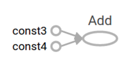
Let's get a little more complex and add our two tensor nodes together. Comment out the last line of your code (with the session.run statement) and add the following.

Next level
So far, our code is not terribly exciting because all of our data is hard-coded and no external input is going in. We can accept external input by declaring placeholders. Note that a + b is a shortcut for tf.add(a, b).
Now, we can actually run this on an array of input as well. Try the following:
We can do further computations on the input before printing it out, for example, if we wanted to add and then triple the value.
In TensorFlow, we differentiate between placeholders and variables. Think of placeholders as representing the data coming in, and variables as trainable parameters. These are the things that your graph will adjust on each iteration.
Back to Linear Regression
Let's create a new python file called regression.py. In this file we'll teach our model to fit a set of data points. We're going to be guessing the values of the variables m and b in the equation for a line mx + b where m and b are variables, and x is the input value. Initially we'll assign random or default initial values to m and b and then we'll train it from there. Start with the following code:
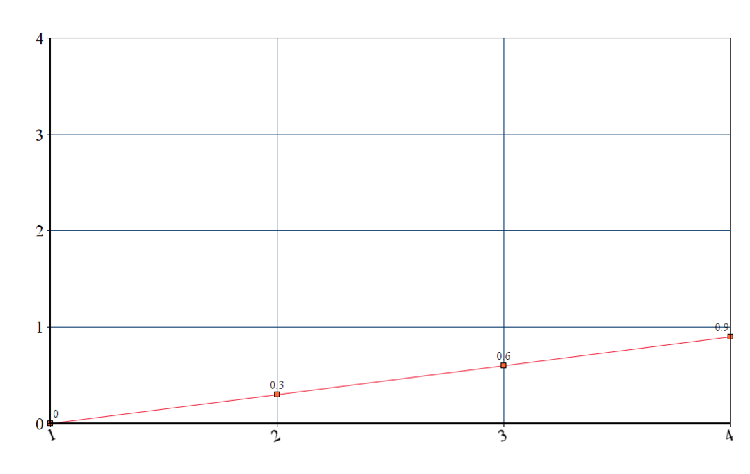
If we were to graph this data, it would look like the following:
x
y
1
0
2
0.30000001
3
0.60000002
4
0.90000004

Now that we have a model, we need actual data to compare it to. Let's say the actual y values are [0, -1, -2, -3]. Knowing that, we can now calculate our 'loss', or how far off we were from the actual values. We do this by taking the difference between each point, squaring that number, then adding all of those numbers together.
y-actual
y-calculated
difference
squared
0
0
0
0
-1
0.3
-1.3
1.69
-2
0.6
-2.6
6.76
-3
0.9
-3.9
15.21
Take the sum of all the numbers in the last column. This yields us a loss value of 23.66. Let's now have TensorFlow do the heavy lifting to calculate this number for us. Add the following code to regression.py.
In an ideal scenario, we can tweak the values of the two variables until the loss is 0. TensorFlow provides optimizer functions that slowly tweak the values of the variables to minimize the loss. The simplest optimizer is called gradient descent. This is how we use it:
Sweet! Notice it got close to the perfect values of 1 and -1 minus some rounding errors.
Classification: Neural Networks using Iris Data
NOTE: You may want to follow TensorFlow for Poets for a simpler (and newer) example.
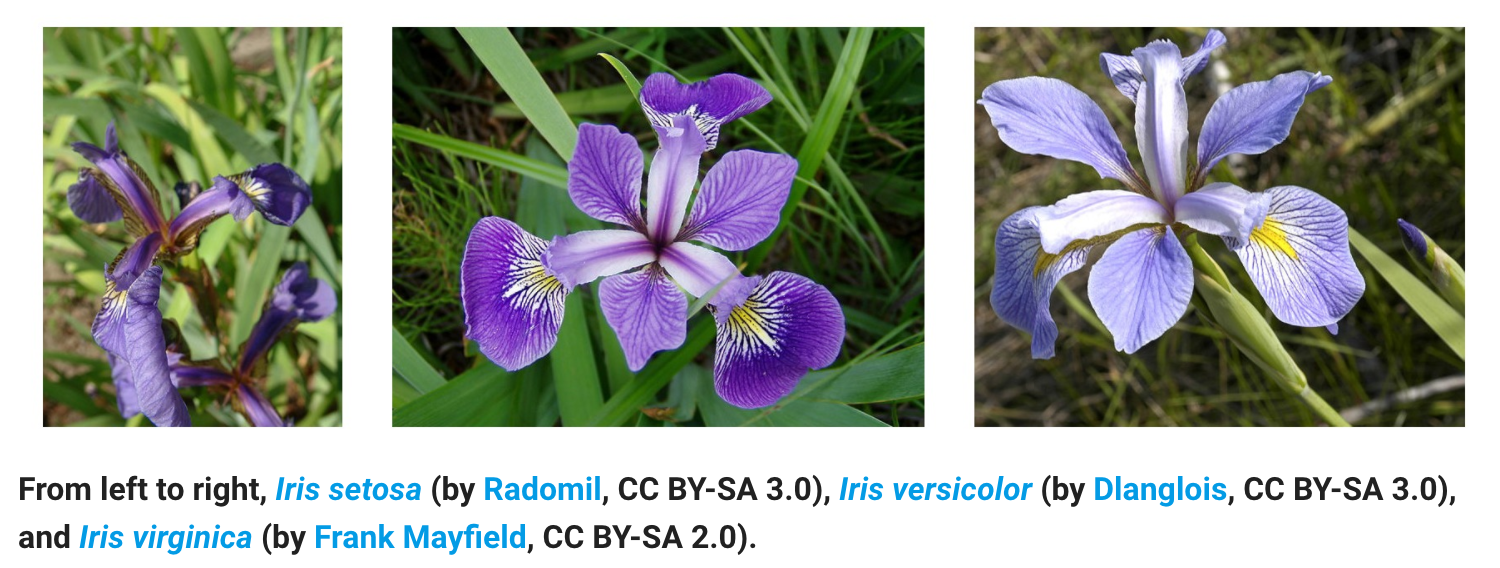
Let's get started on a classification problem where we train a model to detect different species of irises. But first, if you want a brief overview of TensorFlow, watch this video.
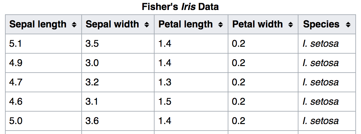
For this code-along we'll go through the example found here. It uses Fisher's iris data set, which measures the length and width of petals and sepals of 3 different species of irises. Sepals in this case are the mini-petals, though on many flowers the sepals are green.

Take a closer look at the data set

Mini-Activity
Get together with a partner. Take note of the ranges and averages of values you see for each of the measurements for each species. If I gave you a random data set of each of the petal and sepal sizes, would you be able to form a good guess as to what the species is?
Let's test this hypothesis. Predict the species for the following data:
sepal length
sepal width
petal length
petal width
species
6.4
3.2
4.5
1.5
?
5.8
3.1
5.0
1.7
?
Keep your guesses handy - we'll train our neural network and see if it agrees.
Getting down to code: Where to start?!
Let's break this down into tasks. Also - take a deep breath - TensorFlow is going to do the heavy lifting for us! :)
Import necessary libraries and declare constants
Import the iris data sets for training and testing
Build the neural network and train it with the training data
Test the accuracy of our model using the testing data set
Use the model to predict the species of our two new specimens (we'll check the answers from our activity)
Here's a breakdown of the code from TensorFlow's site:
1) Import necessary libraries and declare constants
2) Import the iris data sets for training and testing
3) Build the neural network and train it with the training data
4) Test the accuracy of our model using the testing data set
5) Use the model to predict the species of our two new specimens (we'll check the answers from our activity)
So,humans, go back to your guesses. How did you do?
Full code is available on TensorFlow's website.
References and Further reading/watching
Last updated